Hey,

In my last blog post, I talked about rootograms and the new rootogram style that is proposed by Säilynoja et al¹. This new rootogram style puts more emphasis on the discrete nature of count data compared to other rootogram styles. It does this by using discrete visual elements such as point ranges and points instead of lines and filled areas. It also visually looks good and is very compatible with the general plot style followed in bayesplot. In the past two weeks, I have managed to take this idea to a complete implementation and finalised my PR about it, as I promised myself in the last blog post: adding a discrete option to ppc_rootogram.

The last two weeks were very hectic for me, mainly due to my personal life but also partly because this discrete rootogram required more in-depth thinking than I anticipated. To begin with, I had to travel to Turkey for a couple of days for an Australian visa application, which unfortunately cannot be filled out in Finland, mostly because Finnish people are not required to get a visa to travel to Australia. That made me travel to Turkey for a visa appointment that took only an hour or so. Since I didn’t want to stop working, I tried to work on my way there, at the airport, while staying at my family’s house, and so on. Naturally, these weren’t the most efficient and productive working hours. I am not even mentioning the very deep pain that I had in my right leg that made me unable to sleep, which is now getting better after I had a doctor’s appointment, received exercise instructions to follow and some medication to take. As a combined result of all these things, I wasn’t very productive, but I am glad that I managed to complete rootograms and made them ready to be merged to the main branch.

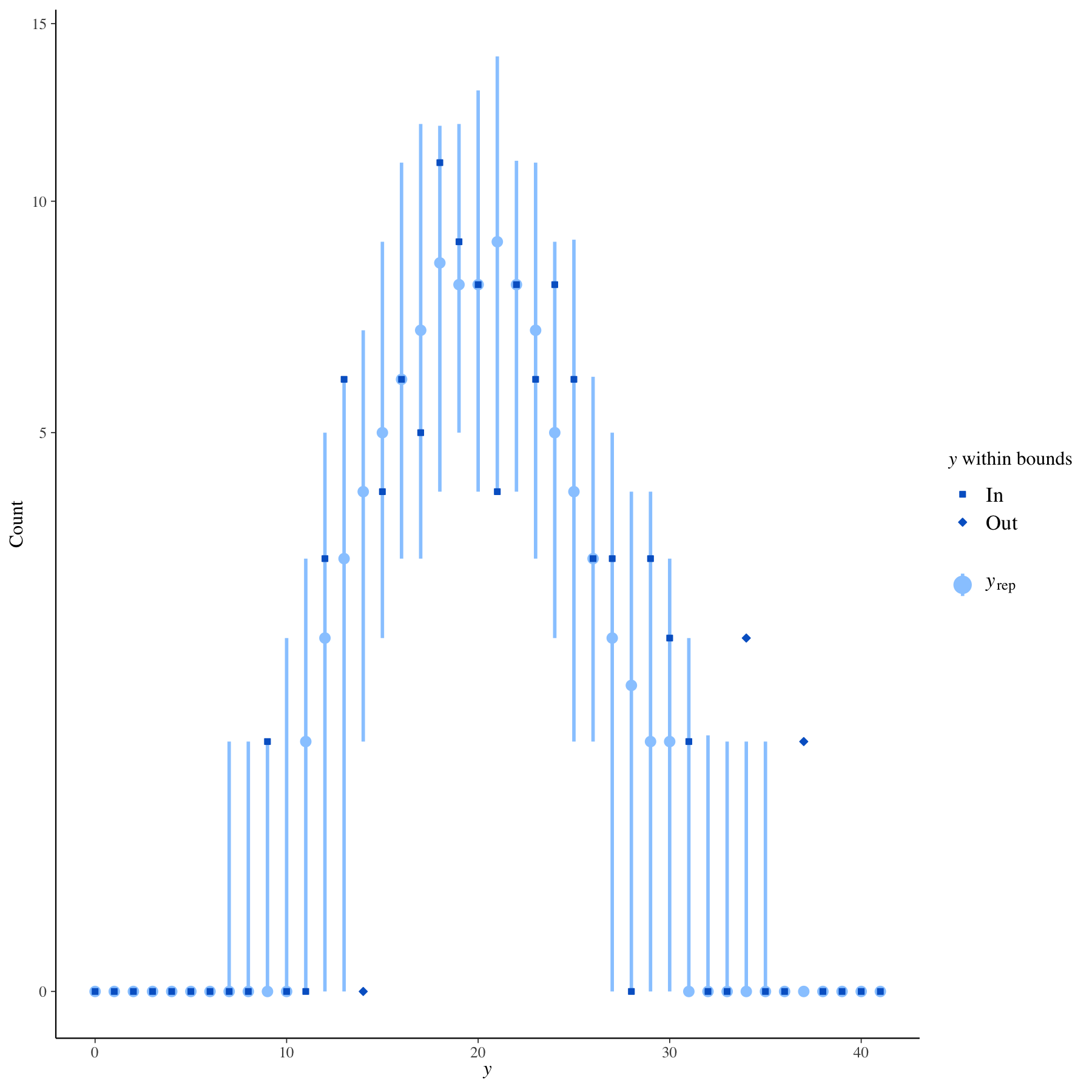
Like I said, the hectic part was mostly about my personal life, but it was also partly related to the rootograms. It turned out that to correctly add a discrete style to a rootogram, there were lots of minor things I needed to consider. For example, in the version proposed in the articles, Teemu opted to use colours as indicators of whether observations lay within the bounds of posterior samples. This is a good idea, which looks nice visually, but it is not compatible with bayesplot. In bayesplot, users are free to pick from colour schemes whose different shades are used to colour different visual elements of the plot. That made having two completely different colours for such a distinction impossible. I also didn’t consider different shades of the same colour to be easy enough to tell apart from each other to be used in such a context. Therefore, we decided to move on with using different shapes as our indicators. Then came the question of which shapes to use. After long discussions, I settled on using squares for within bounds and rhombuses for out-of-bounds points. That being said, I also implemented a new argument called bound_distinct, which is set to true by default and used to control whether the user wants such an indication of within/out of bound points based on the suggestion of Osvaldo A. Martin. When bound_distinct is set to false, all observation points are visualised by squares. This was not the only point of discussion, though. Like I said, in bayesplot, users pick a colour scheme which is then used to colour the plot accordingly. However, it is not always crystal clear how to assign different shades to different parts of the plot. In other rootogram styles, lighter shades are used for observed points while darker shades are used for sampled points. This convention, in my opinion, didn’t make much sense to follow in a discrete style since it is harder to distinguish lighter points laid on top of darker lines. In addition to that, in ppc_interval, which uses point ranges, lighter shades are used for sampled points and darker shades are used for observed points. After a bit of discussion, we decided that this is the logical way to consider the visuality of both options, as well as the fact that we are considering deprecating other rootogram styles after some time, therefore it’s not very sensible to follow their colouring convention. The final part of our discussions was whether to use the median or the mean to determine the centre point of the sampled points. In other rootogram styles, the mean is used to determine the centre, while bounds are based on the quantiles. However, this turned out to be a problematic choice in the context of a discrete style. As we have a style that visualises points discretely and distinguishes whether they lie within bounds or not, we had cases where the observed point is at 0, which is the same as the upper and lower quantiles, but the mean is at 0.04. This meant that the observed point was marked to be within the bounds despite the fact that there weren’t any visual bounds, and the observed point wasn’t on top of the centre point either. It also meant that the centre of our sampled points was out of the bounds, which didn’t make much sense either. Based on these, we decided to use the median to determine centre points. However, we didn’t touch other rootogram styles, and in the documentation and labels of plots, we made it clear that this design choice only applies to the discrete style.

There were lots of discussions and lots of design decisions to be taken; however, finally, the discrete rootograms are ready to be used! My work in the last two weeks, though, wasn’t limited to this. I did a bit of admin work that we discussed before to create a master issue to gather all simple, easy-to-fix issues that can be implemented by people who are new to bayesplot and open source development, which would serve as a soft entry to the world of bayesplot. Under this master issue, I gathered various small sub-issues that newcomers might want to have a look at and pick one to do their first PR: Good First Issues for New Contributors.

In the upcoming weeks, I want to focus more on residual plots. My first goal is to combine ppc_scatter_error_avg and ppc_scatter_error_avg_vs_x to reduce the number of highly similar functions. Then, I plan to move on to the implementation of long-waiting ppc_residual_scatter. If I have time after doing all this, I’ll probably move on to clean up some of the old issues and do some quick PRs. It has been a hectic two weeks; I wish the next two would be at least a little bit calmer. See you in the next blog post!

1. Säilynoja et al. (2025). Recommendations for visual predictive checks in Bayesian workflow. [Online]. Available: https://arxiv.org/abs/2503.01509 ↩︎